Exploring the Species Parameter Database

Overview

fb4package ships with fish4_parameters, a curated database of bioenergetics parameter sets for more than 70 fish species compiled from the primary literature and from Fish Bioenergetics 4.0 (Deslauriers et al. 2017). This vignette shows how to:

Inspect the database structure
Search for species by name or family
Understand the parameter organisation (equations and life stages)
Compare key parameters across species
Use database parameters in a simulation

1. Loading and inspecting the database

data(fish4_parameters)

n_entries <- length(fish4_parameters)
cat("Total entries in database :", n_entries, "\n")
#> Total entries in database : 73
cat("First 12 entries:\n")
#> First 12 entries:
print(head(names(fish4_parameters), 12))
#>  [1] "Alosa pseudoharengus"           "Gadus morhua"                  
#>  [3] "Brevoortia tyrannus"            "Thymallus arcticus baicalensis"
#>  [5] "Clupea harengus"                "Anchoa mitchilli"              
#>  [7] "Hypophthalmichthys nobilis"     "Coregonus hoyi"                
#>  [9] "Pomatomus saltatrix"            "Lepomis macrochirus"           
#> [11] "Salvelinus fontinalis"          "Ameiurus nebulosus"

Each entry is a named list keyed by the species’ scientific name.

2. Database structure

Every entry follows the same hierarchical structure:

fish4_parameters[["Species name"]]
├── species_info        # taxonomic information
├── life_stages         # named list of life-stage parameter sets
│   ├── juvenile        # (or adult, larval, etc.)
│   │   ├── consumption
│   │   ├── respiration
│   │   ├── activity
│   │   ├── sda
│   │   ├── egestion
│   │   ├── excretion
│   │   └── predator    # energy density equation
│   └── adult           # (if present)
└── sources             # literature references

# Inspect a single entry
chinook <- fish4_parameters[["Oncorhynchus tshawytscha"]]

cat("=== Species info ===\n")
#> === Species info ===
print(chinook$species_info)
#> $scientific_name
#> [1] "Oncorhynchus tshawytscha"
#> 
#> $common_name
#> [1] "Chinook salmon (adult)"
#> 
#> $family
#> [1] "Salmonidae"
#> 
#> $order
#> [1] "Salmoniformes"

cat("\n=== Life stages available ===\n")
#> 
#> === Life stages available ===
print(names(chinook$life_stages))
#> [1] "adult"

cat("\n=== Sources ===\n")
#> 
#> === Sources ===
print(chinook$sources)
#> [1] "Stewart & Ibarra 1991; Plumb & Moffit 2015"

3. Searching the database

By scientific name (partial match)

# Find all Oncorhynchus species
onco_keys <- grep("Oncorhynchus", names(fish4_parameters),
                  value = TRUE, ignore.case = TRUE)
cat("Oncorhynchus species in database:\n")
#> Oncorhynchus species in database:
print(onco_keys)
#> [1] "Oncorhynchus tshawytscha" "Oncorhynchus kisutch"    
#> [3] "Oncorhynchus clarki"      "Oncorhynchus gorbuscha"  
#> [5] "Oncorhynchus mykiss"      "Oncorhynchus nerka"

By common name

# Extract all common names and search
common_names <- sapply(fish4_parameters, function(x) {
  x$species_info$common_name %||% NA_character_
})

trout_idx <- grep("trout|salmon|char", common_names,
                  value = FALSE, ignore.case = TRUE)
cat("Salmonid entries (trout / salmon / char):\n")
#> Salmonid entries (trout / salmon / char):
print(common_names[trout_idx])
#>            Salvelinus fontinalis                     Salmo trutta 
#> "Brook Trout (juvenile & adult)"                    "Brown Trout" 
#>           Salvelinus confluentus         Oncorhynchus tshawytscha 
#>             "Bull trout (adult)"         "Chinook salmon (adult)" 
#>             Oncorhynchus kisutch              Oncorhynchus clarki 
#>            "Coho salmon (adult)"                "Cutthroat trout" 
#>             Salvelinus namaycush           Oncorhynchus gorbuscha 
#>             "Lake trout (adult)"            "Pink salmon (adult)" 
#>              Oncorhynchus mykiss               Oncorhynchus nerka 
#>       "Rainbow Trout (juvenile)"         "Sockeye salmon (adult)"

4. Listing available life stages

# Summary of life stages per species
stage_summary <- sapply(fish4_parameters, function(x) {
  paste(names(x$life_stages), collapse = ", ")
})

# Show species that have more than one life stage
multi_stage <- stage_summary[sapply(strsplit(stage_summary, ", "), length) > 1]
cat("Species with multiple life stages (first 8):\n")
#> Species with multiple life stages (first 8):
print(head(multi_stage, 8))
#>           Alosa pseudoharengus                   Gadus morhua 
#> "adult, yearling, yoy, larval"  "juvenile_and_adult, unknown" 
#>                Clupea harengus            Lepomis macrochirus 
#>         "yoy, adult, juvenile"              "adult, juvenile" 
#>              Perca fluviatilus         Engraulis encrasicolus 
#> "1_gram, 100_gram, larval_yoy"  "adult, egg_larval, juvenile" 
#>               Esox masquinongy                Cololabis saira 
#>              "adult, juvenile"              "adult, juvenile"

5. Comparing consumption parameters across species

The maximum consumption rate is governed by:

$C_{\max} = C_A \cdot W^{C_B} \cdot f(T)$

where C_A scales the intercept and C_B the weight exponent. Higher C_A values indicate a higher maximum ration relative to body weight.

# Extract CA, CB, CEQ for all entries (first life stage)
param_table <- do.call(rbind, lapply(names(fish4_parameters), function(sp) {
  entry <- fish4_parameters[[sp]]
  stage <- names(entry$life_stages)[1]
  cons  <- entry$life_stages[[stage]]$consumption

  data.frame(
    Species    = sp,
    Stage      = stage,
    CEQ        = cons$CEQ  %||% NA,
    CA         = cons$CA   %||% NA,
    CB         = cons$CB   %||% NA,
    CTO        = cons$CTO  %||% NA,
    CTM        = cons$CTM  %||% NA,
    stringsAsFactors = FALSE
  )
}))

# Show top 10 by CA (highest maximum ration)
param_table_sorted <- param_table[order(-param_table$CA, na.last = TRUE), ]
knitr::kable(
  head(param_table_sorted[, c("Species", "Stage", "CEQ", "CA", "CB", "CTO", "CTM")], 10),
  caption = "Top 10 entries by CA (maximum consumption coefficient)",
  digits  = 4
)

Top 10 entries by CA (maximum consumption coefficient)
	Species	Stage	CEQ	CA	CB	CTO	CTM
47	Notropis bairdi	unknown	2	4.0330	-1.0589	35.0	41.6
43	Fundulus zebrinus	unknown	2	3.5999	-1.1602	35.0	43.0
8	Coregonus hoyi	adult	2	1.6100	-0.3200	16.8	26.0
26	Coregonus spp.	unknown	2	1.6100	-0.3200	16.8	26.0
31	Coregonus clupeaformis	adult	2	1.6100	-0.3200	16.8	26.0
7	Hypophthalmichthys nobilis	unknown	2	1.5400	-0.2870	26.0	38.0
55	Hypophthalmichthys molitrix	unknown	2	1.5400	-0.2870	29.0	43.0
3	Brevoortia tyrannus	juvenile_and_adult	3	1.2940	-0.3120	28.0	29.0
70	Pomoxis annularis	adult	2	1.2589	-0.6610	24.0	32.0
1	Alosa pseudoharengus	adult	3	0.8464	-0.3000	16.0	18.0

Temperature optima distribution

cto_vals <- na.omit(param_table$CTO)

hist(cto_vals,
     breaks = 15,
     main   = "Consumption temperature optima (CTO)",
     xlab   = "CTO (°C)",
     ylab   = "Number of entries",
     col    = "steelblue",
     border = "white")
abline(v = median(cto_vals), col = "tomato", lwd = 2, lty = 2)
legend("topright", legend = paste("Median =", round(median(cto_vals), 1), "°C"),
       col = "tomato", lty = 2, lwd = 2, bty = "n")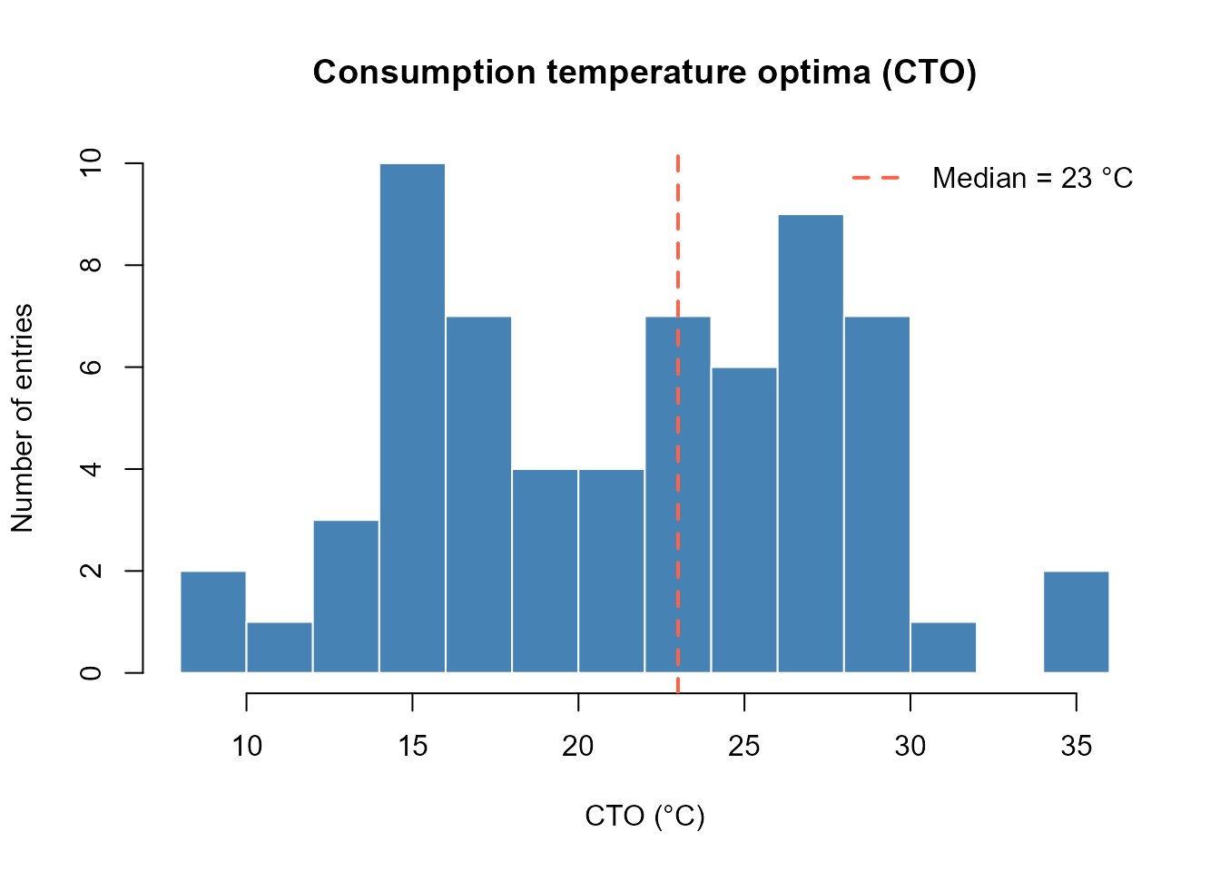

Distribution of consumption temperature optima (CTO) across all database entries.

6. Predator energy density equations

The database includes three equations for predator (fish) energy density:

PREDEDEQ	Form	Parameters
1	Daily interpolation	`ED_data` or `ED_ini` + `ED_end`
2	Piecewise linear in weight	`Alpha1`, `Beta1`, `Alpha2`, `Beta2`, `Cutoff`
3	Power function of weight	`Alpha1`, `Beta1`

prededeq_vals <- sapply(names(fish4_parameters), function(sp) {
  entry <- fish4_parameters[[sp]]
  stage <- names(entry$life_stages)[1]
  entry$life_stages[[stage]]$predator$PREDEDEQ %||% NA
})

cat("Distribution of PREDEDEQ across database:\n")
#> Distribution of PREDEDEQ across database:
print(table(prededeq_vals, useNA = "ifany"))
#> prededeq_vals
#>  1  2  3 
#> 61 11  1

When PREDEDEQ = 1 (the most common), the user must supply ED_ini and ED_end (or a full ED_data vector) since daily energy density varies with season and condition factor. See the Introduction vignette for an example.

7. Building a model directly from the database

# Retrieve brown trout if available, otherwise fall back to first salmonid
target_sp <- grep("Salmo trutta|brown trout",
                  names(fish4_parameters),
                  value = TRUE, ignore.case = TRUE)

if (length(target_sp) == 0) {
  target_sp <- onco_keys[1]   # Fall back to first Oncorhynchus
}
target_sp <- target_sp[1]
cat("Using species:", target_sp, "\n")
#> Using species: Salmo trutta

entry  <- fish4_parameters[[target_sp]]
stage  <- names(entry$life_stages)[1]
params <- entry$life_stages[[stage]]
info   <- entry$species_info
info$life_stage <- stage

# Minimal 60-day setup
days_short <- 1:60
bio_db <- Bioenergetic(
  species_params     = params,
  species_info       = info,
  environmental_data = list(
    temperature = data.frame(Day = days_short,
                             Temperature = 10 + 3 * sin(pi * days_short / 60))
  ),
  diet_data = list(
    proportions = data.frame(Day = days_short, Invertebrates = 1),
    prey_names  = "Invertebrates",
    energies    = data.frame(Day = days_short, Invertebrates = 2800)
  ),
  simulation_settings = list(initial_weight = 50, duration = 60)
)

# Supply energy density bounds for PREDEDEQ = 1
bio_db$species_params$predator$ED_ini <- 4000
bio_db$species_params$predator$ED_end <- 4500

res_db <- run_fb4(bio_db,
                  fit_to    = "Weight",
                  fit_value = 80,
                  strategy  = "binary_search",
                  verbose   = FALSE)

cat(sprintf("Estimated p : %.4f  |  Final weight : %.1f g\n",
            res_db$summary$p_value,
            res_db$summary$final_weight))
#> Estimated p : 0.6651  |  Final weight : 80.0 g

8. Adding a custom species

If your species is not in the database, supply parameters manually in the same list structure and pass them directly to Bioenergetic(). See the Introduction vignette for a full example with Stewart & Ibarra (1991) parameters for Chinook salmon.

References

Deslauriers D, Chipps SR, Breck JE, Rice JA, Madenjian CP (2017). Fish Bioenergetics 4.0: An R-Based Modeling Application. Fisheries 42(11):586–596. https://doi.org/10.1080/03632415.2017.1377558

Hanson PC, Johnson TB, Schindler DE, Kitchell JF (1997). Fish Bioenergetics 3.0. University of Wisconsin Sea Grant Institute, Report WISSG-97-250.

Hans Ttito

2026-03-29