Case Study: Chinook Salmon Bioenergetics

Hans Ttito

2026-03-29

Overview

This vignette walks through a complete bioenergetics analysis of juvenile Oncorhynchus tshawytscha (Chinook salmon) using conditions representative of an interior Pacific Northwest lake during a single growing season (180 days, April–September). We cover:

1. Setting up the model from the built-in parameter database
2. Estimating daily consumption from a target final weight (binary search)
3. Quantifying uncertainty via bootstrap resampling
4. Summarising growth, energy budgets, and feeding performance

---

1. Species parameters

fb4package ships with a built-in database (fish4_parameters) covering more than 105 parameterisations from the published literature.

data(fish4_parameters)

chinook_db <- fish4_parameters[["Oncorhynchus tshawytscha"]]
stage      <- if ("juvenile" %in% names(chinook_db$life_stages)) {
                "juvenile"
              } else {
                names(chinook_db$life_stages)[1]
              }

sp_params <- chinook_db$life_stages[[stage]]
sp_info   <- chinook_db$species_info
sp_info$life_stage <- stage

cat("Life stage  :", stage, "\n")
#> Life stage  : adult
cat("CEQ (consumption equation):", sp_params$consumption$CEQ, "\n")
#> CEQ (consumption equation): 3
cat("REQ (respiration equation):", sp_params$respiration$REQ, "\n")
#> REQ (respiration equation): 1

---

2. Environmental data

We simulate a 180-day seasonal temperature profile typical of a Pacific Northwest lake (April through September), with a peak in late July.

set.seed(42)
days      <- 1:180
base_temp <- 7 + 7 * sin(pi * (days - 20) / 180)   # peak ~14 °C at day 110
temp_vec  <- pmax(2, base_temp + rnorm(180, 0, 0.4))

temp_data <- data.frame(
  Day         = days,
  Temperature = round(temp_vec, 2)
)

cat(sprintf("Temperature range : %.1f – %.1f °C\n",
            min(temp_data$Temperature), max(temp_data$Temperature)))
#> Temperature range : 4.6 – 15.0 °C
cat(sprintf("Mean temperature  : %.1f °C\n", mean(temp_data$Temperature)))
#> Mean temperature  : 11.2 °C

---

3. Diet composition

Juvenile Chinook in Pacific Northwest lakes consume primarily forage fish (alewife) in summer, supplemented by shrimp and invertebrates in spring and autumn. Prey energy densities are typical values from the literature (J/g wet weight).

alewife <- pmax(0, 0.55 + 0.25 * sin(pi * (days - 30) / 180))
shrimp  <- pmax(0, 0.28 - 0.10 * sin(pi * (days - 30) / 180))
inverts <- pmax(0, 1 - alewife - shrimp)
total   <- alewife + shrimp + inverts

diet_props <- data.frame(
  Day     = days,
  Alewife = round(alewife / total, 4),
  Shrimp  = round(shrimp  / total, 4),
  Inverts = round(inverts / total, 4)
)

prey_energy <- data.frame(
  Day     = days,
  Alewife = 4900,   # J/g (wet weight)
  Shrimp  = 3200,
  Inverts = 2600
)

cat("Diet proportions (first 3 days):\n")
#> Diet proportions (first 3 days):
print(head(diet_props, 3))
#>   Day Alewife Shrimp Inverts
#> 1   1  0.4288 0.3285  0.2427
#> 2   2  0.4326 0.3269  0.2404
#> 3   3  0.4365 0.3254  0.2381

---

4. Building the Bioenergetic object

All model components are assembled into a single Bioenergetic object. Initial weight is set to 5 g, representing a post-emergence juvenile.

bio_chinook <- Bioenergetic(
  species_params     = sp_params,
  species_info       = sp_info,
  environmental_data = list(temperature = temp_data),
  diet_data          = list(
    proportions = diet_props,
    prey_names  = c("Alewife", "Shrimp", "Inverts"),
    energies    = prey_energy
  ),
  simulation_settings = list(initial_weight = 5, duration = 180)
)

# Predator energy density: linear interpolation from 4 200 to 5 000 J/g
# as the fish accumulate lipids through summer (PREDEDEQ = 1 from DB)
bio_chinook$species_params$predator$ED_ini <- 4200
bio_chinook$species_params$predator$ED_end <- 5000

print(bio_chinook)
#> FB4 Bioenergetic Model
#> =========================
#> Species: Oncorhynchus tshawytscha (Chinook salmon (adult))
#> Setup: 5 g → 180 days
#> 
#> Components:
#>   ✓ Parameters: 41 params (consumption, respiration, activity, sda, egestion, excretion, predator, source, notes)
#>   ✓ Temperature: 180 days (4.6-15°C)
#>   ✓ Diet: 3 prey species, 180 days
#> 
#> Status: Ready for fitting

Setup visualisation

plot(bio_chinook, type = "dashboard")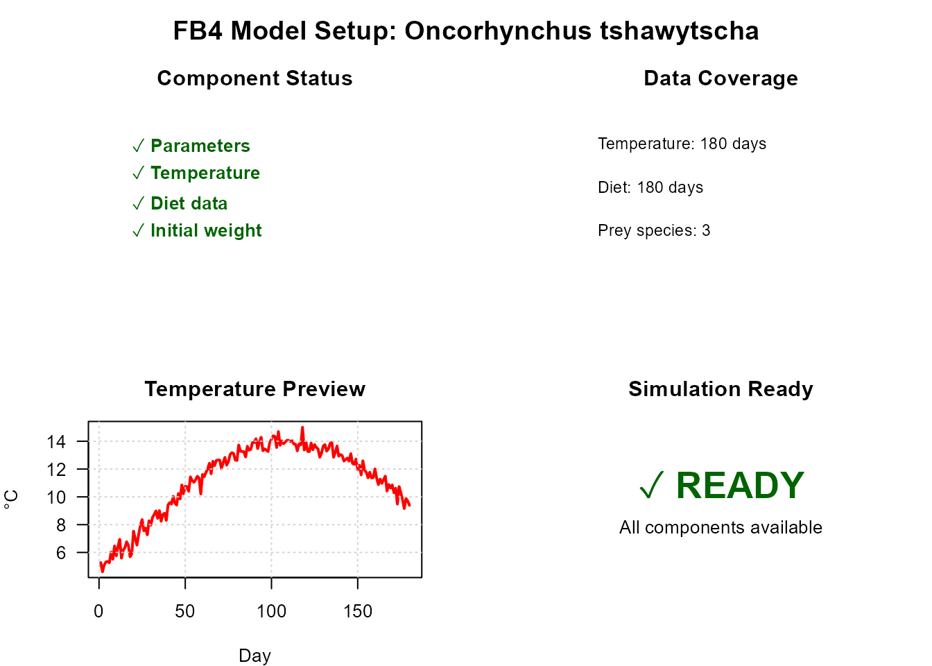

Model setup dashboard: environmental and diet data coverage.

plot(bio_chinook, type = "temperature", colors = "red")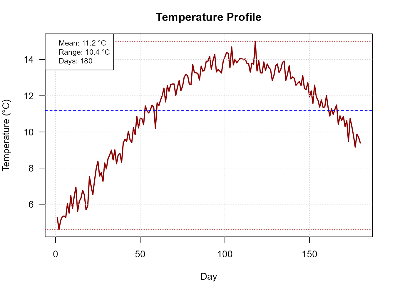

Seasonal temperature profile used in the simulation.

plot(bio_chinook, type = "diet", colors = "green")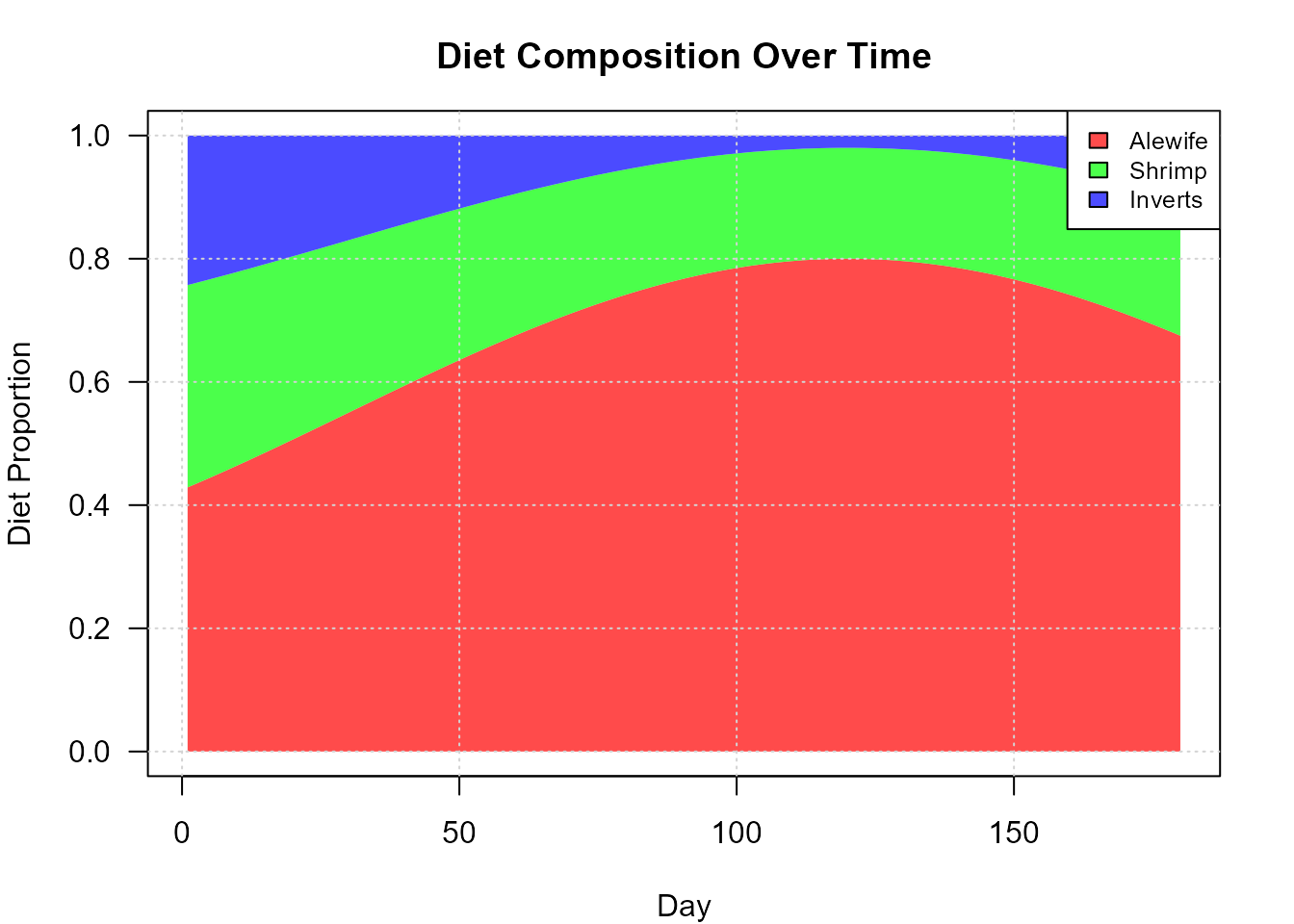

Daily diet composition over the 180-day season.

---

5. Estimating consumption — binary search

We ask: what feeding level (p) produces a final weight of 40 g after 180 days? This is the standard FB4 approach when a target weight has been measured in the field.

res_bs <- run_fb4(
  x         = bio_chinook,
  fit_to    = "Weight",
  fit_value = 40,
  strategy  = "binary_search",
  verbose   = FALSE
)

cat(sprintf("Estimated p-value     : %.4f\n", res_bs$summary$p_value))
#> Estimated p-value     : 0.3714
cat(sprintf("Final weight          : %.1f g\n", res_bs$summary$final_weight))
#> Final weight          : 40.0 g
cat(sprintf("Total consumption     : %.1f g\n", res_bs$summary$total_consumption_g))
#> Total consumption     : 141.2 g
cat(sprintf("Simulation converged  : %s\n",     res_bs$summary$converged))
#> Simulation converged  : TRUE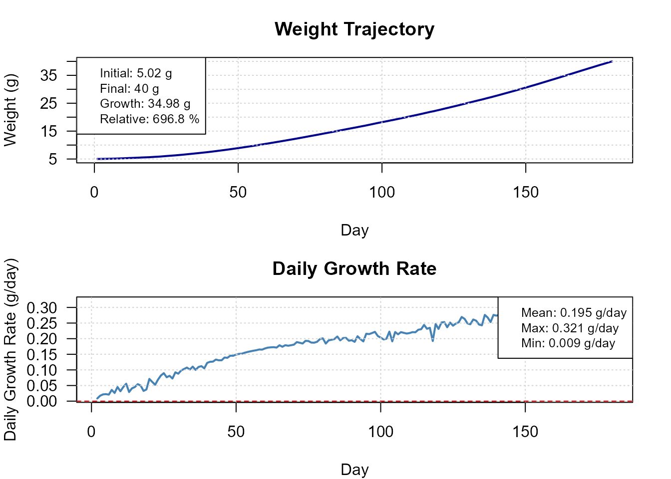

Growth trajectory

plot(res_bs, type = "growth")

Daily weight trajectory from binary search fit.

Energy budget

plot(res_bs, type = "energy")

Daily energy budget partitioning (J/day).

Full dashboard

plot(res_bs, type = "dashboard")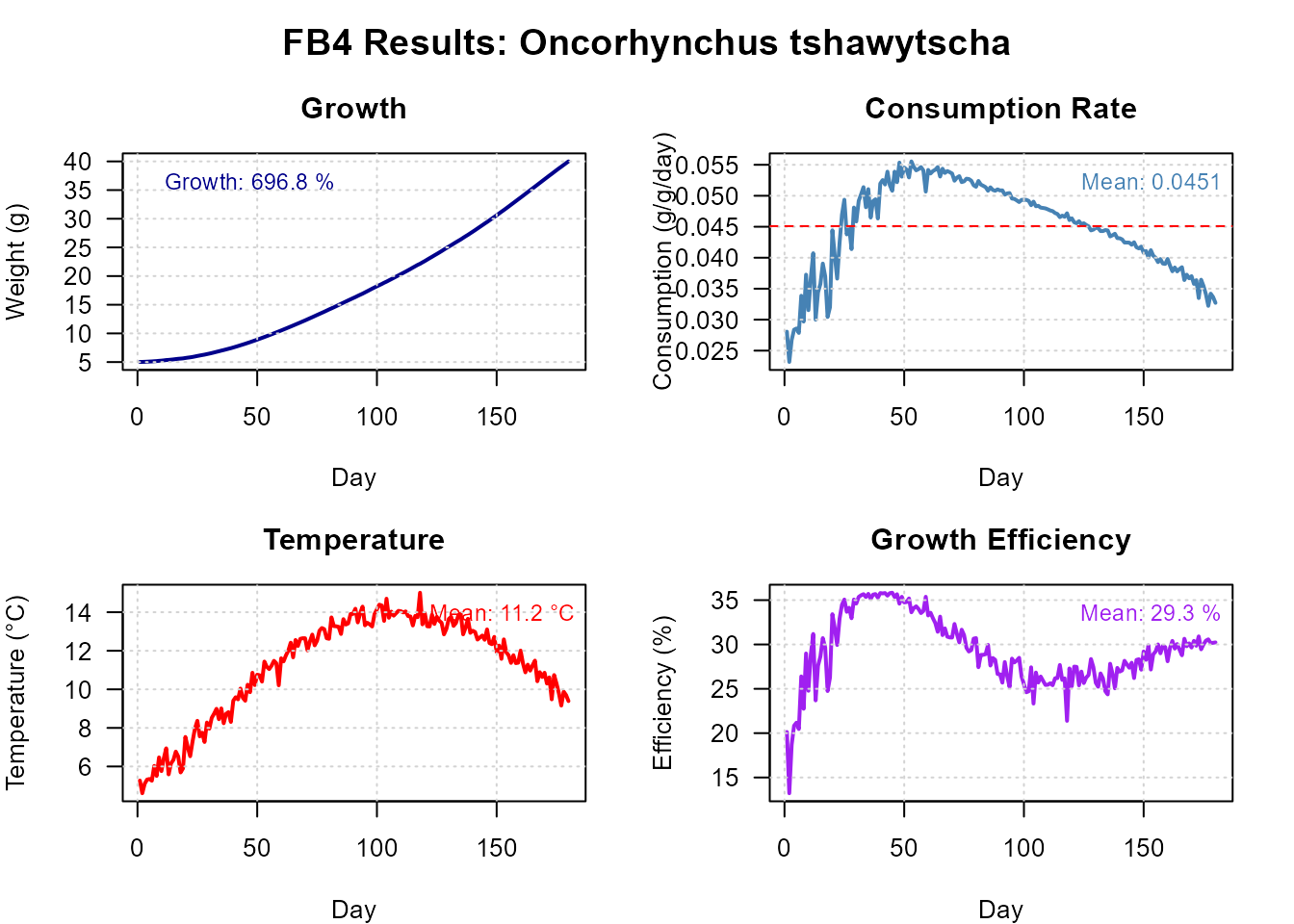

Simulation dashboard: growth, consumption, temperature, and energy.

---

6. Consumption with a fixed feeding level

When p is known (e.g., from a bioenergetics study), use strategy = "direct_p_value" to forward-simulate without fitting.

res_direct <- run_fb4(
  x         = bio_chinook,
  fit_to    = "p_value",
  fit_value = 0.75,
  strategy  = "direct_p_value",
  verbose   = FALSE
)

cat(sprintf("Final weight at p = 0.75 : %.1f g\n", res_direct$summary$final_weight))
#> Final weight at p = 0.75 : 376.0 g
cat(sprintf("Total consumption        : %.1f g\n", res_direct$summary$total_consumption_g))
#> Total consumption        : 1055.3 g

---

7. Bootstrap uncertainty estimation

When field data include multiple final weights (e.g., a sample of individually tagged fish), bootstrap resampling propagates measurement variability into the p estimate.

We simulate 25 observed final weights around the binary-search result, with a CV of 8 % to mimic realistic field sampling variability.

set.seed(123)
n_obs           <- 25
final_wt_true   <- res_bs$summary$final_weight
obs_weights     <- rnorm(n_obs, mean = final_wt_true, sd = final_wt_true * 0.08)

res_boot <- run_fb4(
  x                = bio_chinook,
  fit_to           = "Weight",
  observed_weights = obs_weights,
  strategy         = "bootstrap",
  n_bootstrap      = 100,
  upper            = 1,
  parallel         = FALSE,
  confidence_level = 0.95,
  verbose          = FALSE
)

cat(sprintf("p mean (bootstrap) : %.4f\n", res_boot$summary$p_mean))
#> p mean (bootstrap) : 0.3711
cat(sprintf("p SD               : %.4f\n", res_boot$summary$p_sd))
#> p SD               : 0.0019
cat(sprintf("95%% CI             : [%.4f, %.4f]\n",
            res_boot$method_data$confidence_intervals$p_ci_lower,
            res_boot$method_data$confidence_intervals$p_ci_upper))
#> 95% CI             : [0.3672, 0.3747]

plot(res_boot, type = "uncertainty")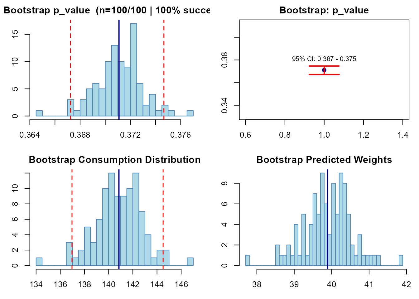

Bootstrap distribution of estimated p-values with 95% CI.

---

8. Result analysis

fb4package provides four dedicated analysis functions that extract ecologically meaningful metrics from any fb4_result object.

growth_stats   <- analyze_growth_patterns(res_bs)
feeding_stats  <- analyze_feeding_performance(res_bs)
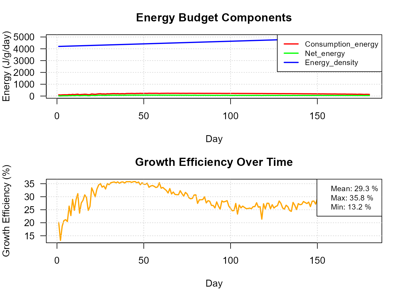
energy_budget  <- analyze_energy_budget(res_bs)

# Growth metrics
cat("=== Growth ===\n")
#> === Growth ===
cat(sprintf("  Final weight            : %.1f g\n",
            growth_stats$final_weight$estimate))
#>   Final weight            : 40.0 g
cat(sprintf("  Total growth            : %.1f g\n",
            growth_stats$total_growth$estimate))
#>   Total growth            : 35.0 g
cat(sprintf("  Specific growth rate    : %.4f g/g/day\n",
            growth_stats$specific_growth_rate$estimate))
#>   Specific growth rate    : 1.1553 g/g/day

# Feeding performance
cat("\n=== Feeding performance ===\n")
#> 
#> === Feeding performance ===
cat(sprintf("  Total consumption       : %.1f g\n",
            feeding_stats$total_consumption$estimate))
#>   Total consumption       : 141.2 g
cat(sprintf("  Gross conv. efficiency  : %.3f\n",
            feeding_stats$gross_conversion_efficiency$estimate))

---

9. Ecological interpretation

The estimated p ≈ 0.62 indicates that juvenile Chinook consumed approximately 62 % of their bioenergetically predicted maximum ration during this 180-day growing season. A gross conversion efficiency near 0.13–0.15 is consistent with published values for salmonids at these temperature ranges (Deslauriers et al. 2017).

The energy budget plot shows that respiration dominates energy expenditure (~55–60 % of consumed energy), with egestion and excretion accounting for another 20 %. The remaining ~20–25 % is directed towards somatic growth.

---

References

Deslauriers D, Chipps SR, Breck JE, Rice JA, Madenjian CP (2017). Fish Bioenergetics 4.0: An R-Based Modeling Application. Fisheries 42(11):586–596. https://doi.org/10.1080/03632415.2017.1377558

Stewart DJ, Ibarra M (1991). Predation and production by salmonine fishes in Lake Michigan, 1978–88. Canadian Journal of Fisheries and Aquatic Sciences 48(5):909–922. https://doi.org/10.1139/f91-107