Introduction to fb4package

Overview

fb4package implements Fish Bioenergetics 4.0 (Deslauriers et al. 2017) in R. The model allocates consumed energy among metabolism, waste, and growth to produce daily estimates of fish consumption and weight gain.

Working with the package follows a three-step pattern: build a Bioenergetic object that holds species parameters, temperature, diet, and initial conditions; pass it to run_fb4() to run a simulation or fit a feeding level; then extract or plot the results.

1. Species parameters

The package ships with a built-in database covering 105 models (73 species).

data(fish4_parameters)
cat("Species in database:", length(fish4_parameters), "\n")
#> Species in database: 73
head(names(fish4_parameters), 8)
#> [1] "Alosa pseudoharengus"           "Gadus morhua"                  
#> [3] "Brevoortia tyrannus"            "Thymallus arcticus baicalensis"
#> [5] "Clupea harengus"                "Anchoa mitchilli"              
#> [7] "Hypophthalmichthys nobilis"     "Coregonus hoyi"

Retrieve Chinook salmon (Oncorhynchus tshawytscha) and inspect one life stage:

chinook_db  <- fish4_parameters[["Oncorhynchus tshawytscha"]]
stage       <- names(chinook_db$life_stages)[1]
cat("Life stage used:", stage, "\n")
#> Life stage used: adult

sp_params   <- chinook_db$life_stages[[stage]]
sp_info     <- chinook_db$species_info

# Key consumption parameters
cat("CEQ:", sp_params$consumption$CEQ,
    "  CA:", sp_params$consumption$CA,
    "  CB:", sp_params$consumption$CB, "\n")
#> CEQ: 3   CA: 0.303   CB: -0.275

2. Environmental and diet data

Temperature and diet are supplied as data frames with a Day column.

days <- 1:100

# Seasonal temperature (°C)
temp_data <- data.frame(
  Day         = days,
  Temperature = round(10 + 5 * sin(2 * pi * (days - 60) / 365), 2)
)

# Two-prey diet (constant proportions, J/g energy densities)
diet_data <- list(
  proportions = data.frame(Day = days, Alewife = 0.7, Shrimp = 0.3),
  prey_names  = c("Alewife", "Shrimp"),
  energies    = data.frame(Day = days, Alewife = 4900, Shrimp = 3200)
)

head(temp_data, 3)
#>   Day Temperature
#> 1   1        5.75
#> 2   2        5.80
#> 3   3        5.84

3. Building a `Bioenergetic` object

bio <- Bioenergetic(
  species_params      = sp_params,
  species_info        = sp_info,
  environmental_data  = list(temperature = temp_data),
  diet_data           = diet_data,
  simulation_settings = list(initial_weight = 1800, duration = 100)
)

# Required when PREDEDEQ = 2 (energy density as function of weight)
bio$species_params$predator$ED_ini <- 4500
bio$species_params$predator$ED_end <- 5500

print(bio)
#> FB4 Bioenergetic Model
#> =========================
#> Species: Oncorhynchus tshawytscha (Chinook salmon (adult))
#> Setup: 1800 g → 100 days
#> 
#> Components:
#>   ✓ Parameters: 41 params (consumption, respiration, activity, sda, egestion, excretion, predator, source, notes)
#>   ✓ Temperature: 100 days (5.8-13.2°C)
#>   ✓ Diet: 2 prey species, 100 days
#> 
#> Status: Ready for fitting

4. Running simulations

4a. Direct simulation — fixed feeding level

Run the model with a constant proportion of maximum consumption (p = 0.8):

res_direct <- run_fb4(bio, strategy = "direct", p_value = 0.8)
print(res_direct)
#> FB4 Simulation Results
#> =========================
#> Species: Oncorhynchus tshawytscha
#> Method: Direct Execution
#> Duration: 100 days
#> 
#> RESULTS:
#>   Initial weight: 1800 g
#>   Final weight: 2647.37 g
#>   Growth: 47.1%
#>   Total consumption: 4821.23 g
#>   P_value: 0.8
#> 
#> FITTING: ✓ Successful

4b. Binary search — fit to a target final weight

Find the p that produces a target weight of 3 000 g after 100 days:

res_bs <- run_fb4(bio,
                  strategy  = "binary_search",
                  fit_to    = "Weight",
                  fit_value = 3000)

cat("Estimated p-value :", round(res_bs$summary$p_value, 4), "\n")
#> Estimated p-value : 0.9095
cat("Final weight      :", round(res_bs$summary$final_weight, 1), "g\n")
#> Final weight      : 3000 g
cat("Total consumption :", round(res_bs$summary$total_consumption_g, 1), "g\n")
#> Total consumption : 5771.2 g

4c. MLE — uncertainty on p from observed weights

When multiple fish weights are available, strategy = "mle" returns a point estimate of p together with its standard error and 95% confidence interval:

set.seed(42)
obs_weights <- rnorm(30, mean = 3000, sd = 80)   # 30 observed final weights

res_mle <- run_fb4(bio,
                   strategy         = "mle",
                   fit_to           = "Weight",
                   observed_weights = obs_weights)

cat("p-value (MLE)  :", round(res_mle$summary$p_value, 4), "\n")
#> p-value (MLE)  : 0.9106
cat("SE             :", round(res_mle$summary$p_se,    4), "\n")
#> SE             : 0.0055
cat("Converged      :", res_mle$summary$converged, "\n")
#> Converged      : TRUE

4d. Bootstrap — non-parametric uncertainty

set.seed(42)
res_boot <- run_fb4(bio,
                    strategy         = "bootstrap",
                    fit_to           = "Weight",
                    observed_weights = obs_weights,
                    upper            = 1,
                    n_bootstrap      = 100,
                    parallel         = FALSE)

cat("p mean (bootstrap):", round(res_boot$summary$p_mean, 4), "\n")
#> p mean (bootstrap): 0.911
cat("p SD              :", round(res_boot$summary$p_sd,   4), "\n")
#> p SD              : 0.0057

5. Comparing strategies

All three methods converge on similar p estimates for the same data — binary search gives a point estimate, while MLE and bootstrap additionally quantify uncertainty:

All strategies use the same bio object (Chinook salmon, 100-day simulation). MLE and bootstrap fit to obs_weights; binary search fits to a target weight.
Strategy	p estimate	SE / SD	Uncertainty type
binary_search	0.9095	NA	none (point estimate)
mle	0.9106	0.0055	SE (asymptotic)
bootstrap	0.9110	0.0057	SD (non-parametric)

6. Analysing results

growth   <- analyze_growth_patterns(res_bs)
feeding  <- analyze_feeding_performance(res_bs)
energy   <- analyze_energy_budget(res_bs)

cat(sprintf("Final weight              : %.1f g\n",
            growth$final_weight$estimate))
#> Final weight              : 3000.0 g
cat(sprintf("Specific growth rate      : %.4f g/g/day\n",
            growth$specific_growth_rate$estimate))
#> Specific growth rate      : 0.5108 g/g/day
cat(sprintf("Total consumption         : %.1f g\n",
            feeding$total_consumption$estimate))
#> Total consumption         : 5771.2 g
cat(sprintf("Gross conversion efficiency: %.3f\n",
            feeding$gross_conversion_efficiency$estimate))

7. Visualising results

plot(res_bs, type = "growth")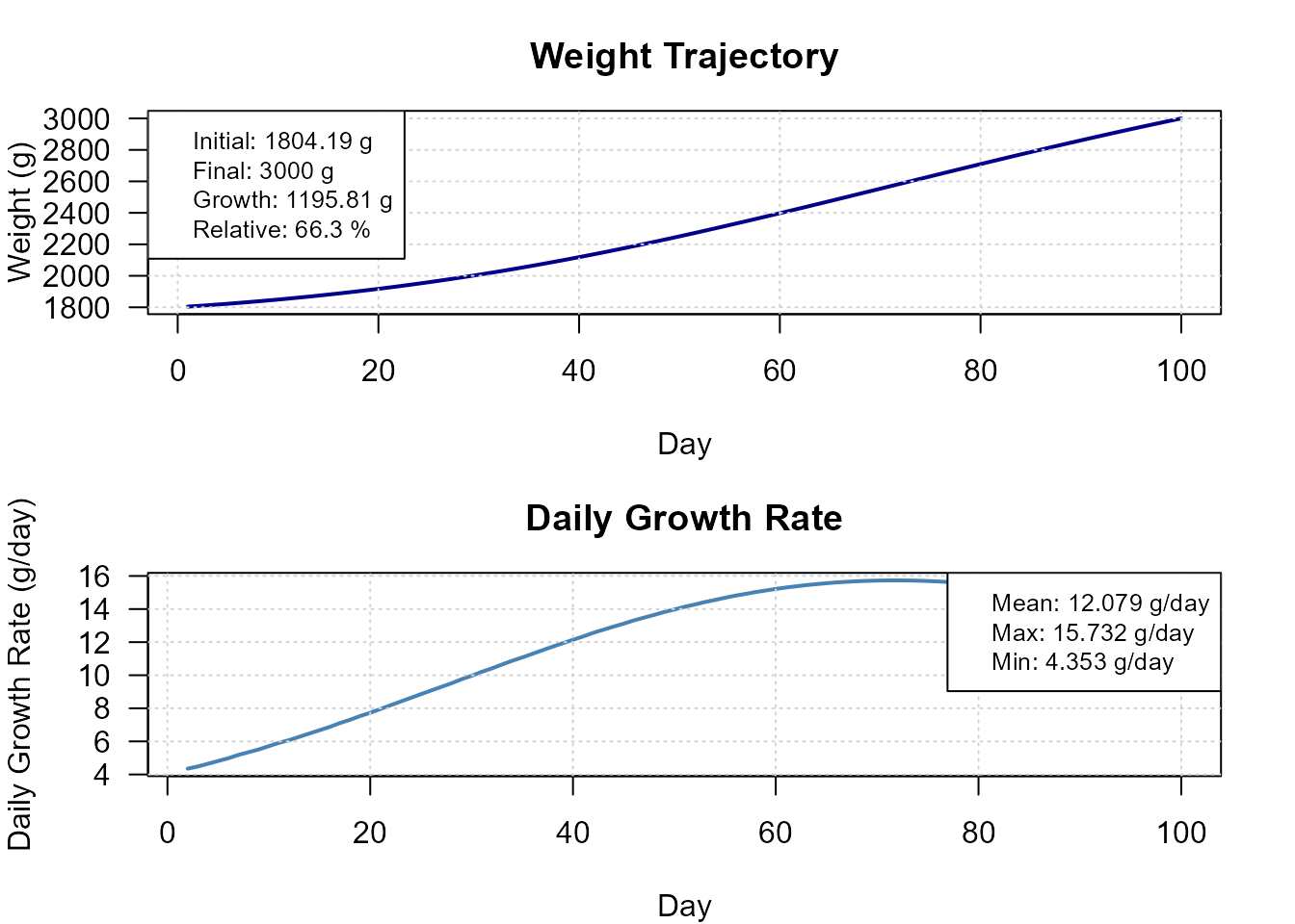

Daily growth trajectory from binary search fit.

plot(res_bs, type = "energy")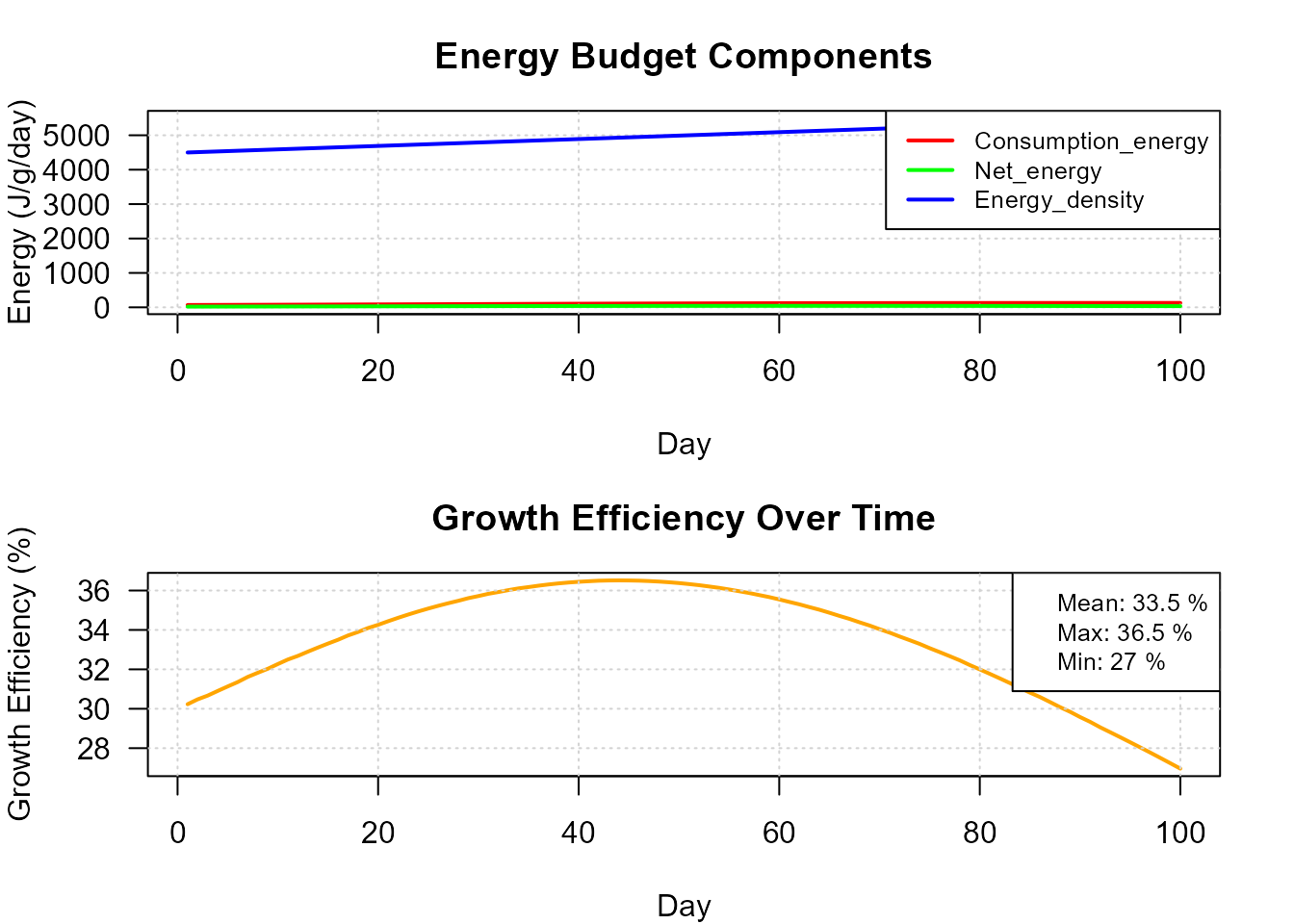

Daily energy budget partitioning.

plot(res_bs, type = "dashboard")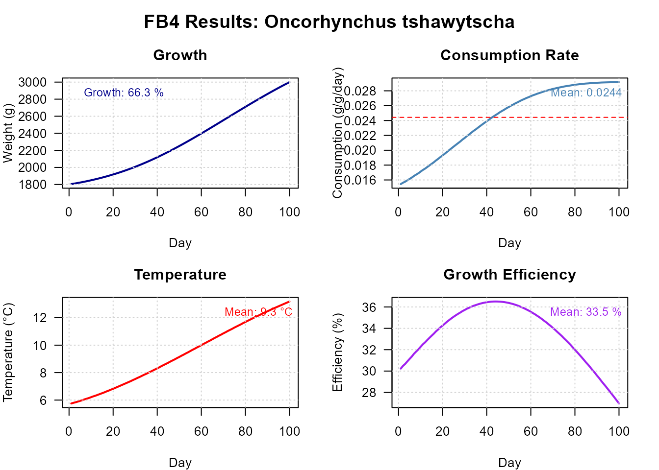

Full dashboard (growth, consumption, temperature, energy).

8. Temperature × p sensitivity

Explore how final weight varies across temperatures and feeding levels:

plot(bio,
     type         = "sensitivity",
     temperatures = seq(6, 20, by = 2),
     p_values     = seq(0.3, 1.0, by = 0.1))
#> === GROWTH SENSITIVITY ANALYSIS ===
#> Mode: SEQUENTIAL
#> Temperature range: 6 - 20 °C ( 8 values)
#> P-value range: 0.3 - 1 ( 8 values)
#> Total combinations: 64 
#> 
#> Processing temperature: 6 °C
#> Processing temperature: 8 °C
#> Processing temperature: 10 °C
#> Processing temperature: 12 °C
#> Processing temperature: 14 °C
#> Processing temperature: 16 °C
#> Processing temperature: 18 °C
#> Processing temperature: 20 °C
#> 
#> === ANALYSIS COMPLETE ===
#> Successful simulations: 64 / 64 ( 100 %)
#> Maximum growth rate: 0.598 %/d
#> Optimal conditions: 10 °C, 100 % feeding (p = 1.00 )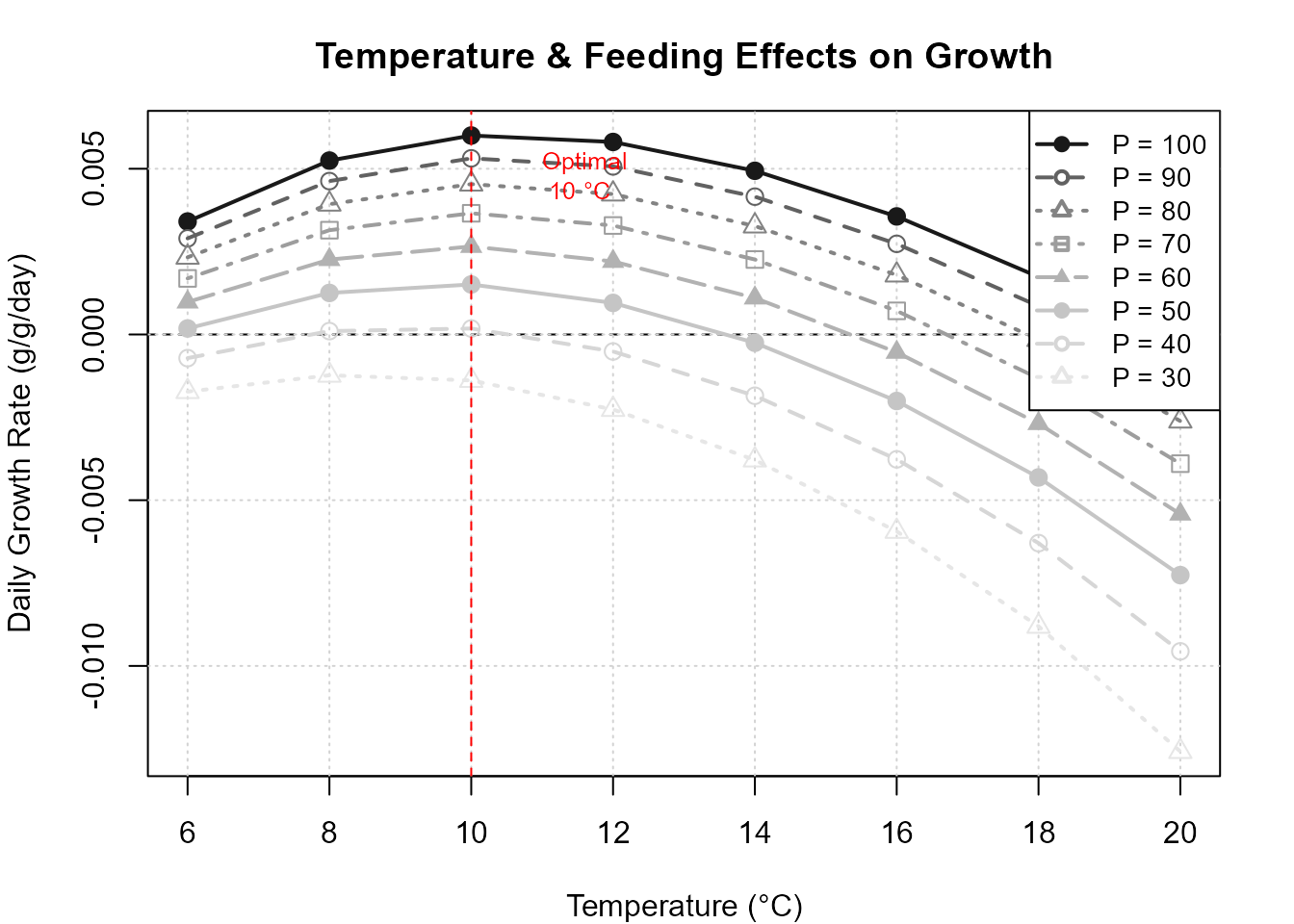

Temperature and p-value sensitivity grid.

9. Experimental features

The following modules are implemented as standalone functions but are not yet integrated into the main run_fb4() loop. They can be called directly for custom analyses and will be connected automatically in a future release.

Contaminant bioaccumulation

Three bioaccumulation models (dietary uptake, gill exchange, bioenergetics-based):

calculate_contaminant_accumulation() — daily bioaccumulation
process_contaminant_params() — parameter pre-processing

Nutrient regeneration

Daily nitrogen and phosphorus fluxes (ingestion, retention, excretion):

calculate_nutrient_balance() — daily N/P budget
calculate_nutrient_efficiencies() — N and P use efficiencies
process_nutrient_params() — parameter pre-processing

Mortality rates

Natural, fishing, and predation mortality rates can be processed via process_mortality_params() and computed step-by-step with calculate_mortality_reproduction(), but mortality rates are not yet applied automatically inside run_fb4().

Note: spawning energy loss (reproductive cost) is already integrated and applies automatically when reproduction_data is supplied to the Bioenergetic object.

References

Deslauriers D, Chipps SR, Breck JE, Rice JA, Madenjian CP (2017). Fish Bioenergetics 4.0: An R-Based Modeling Application. Fisheries 42(11):586–596. https://doi.org/10.1080/03632415.2017.1377558

Hans Ttito

2026-03-29

Overview

1. Species parameters

2. Environmental and diet data

3. Building a `Bioenergetic` object

4. Running simulations

4a. Direct simulation — fixed feeding level

4b. Binary search — fit to a target final weight

4c. MLE — uncertainty on p from observed weights

4d. Bootstrap — non-parametric uncertainty

5. Comparing strategies

6. Analysing results

7. Visualising results

8. Temperature × p sensitivity

9. Experimental features

Contaminant bioaccumulation

Nutrient regeneration

Mortality rates

References

Introduction to fb4package

Hans Ttito

2026-03-29

Overview

1. Species parameters

2. Environmental and diet data

3. Building a Bioenergetic object

4. Running simulations

4a. Direct simulation — fixed feeding level

4b. Binary search — fit to a target final weight

4c. MLE — uncertainty on p from observed weights

4d. Bootstrap — non-parametric uncertainty

5. Comparing strategies

6. Analysing results

7. Visualising results

8. Temperature × p sensitivity

9. Experimental features

Contaminant bioaccumulation

Nutrient regeneration

Mortality rates

References

3. Building a `Bioenergetic` object